
| url | Bias Specific | article | cleaned |
|---|---|---|---|
| Loading ITables v2.3.0 from the internet... (need help?) |
Neural Networks
Introduction
Neural Networks are supervised machine learning models which draw inspiration from the human brain. Specifically, they attempt to model how the neurons in the human brain work. Although this won’t serve any justice to the true complexities of the biology behind neurons, the general extension to machine learning can be explained.
- Neurons are connected to each other.
- They send signals (or information) to each other.
- The connections between the neurons form a network of neurons.
- Neurons will fire (or send an electrical pulse) when a threshold is reached:
- Connected neurons will receive that pulse.
- In turn, the pulse may bring the connected neurons to their threshold causing them to fire.
- This continues within the layers of connected nodes, propagating information through the network.
Research on algorithmically modeling and implementing the structure of the brain into a computational asset has been ongoing for decades [1]. There have been periods of stagnation and periods of brilliant breakthroughs culminating in the diverse neural network architectures available today. In fact, one notable problem accounted for both a momentary lag and then an explosion, the XOR Problem. The framework can be described as a binary operation that takes two binary inputs and produces a binary output, where the output of the operation is 1 only when the inputs are different. The initial issue was that primitive neural networks, represented by a single-layer perceptron (or artificial neuron) failed to solve this problem due to the data not being linearly separable. However, the breakthrough occurred when feedforward neural networks (or multi-layer perceptron) were developed [2]. A feedforward neural network has an input layer which takes the input, a hidden layer which applies non-linear activation functions to create transformed features which aid in separating classes, and an output layer for the result.
The Breakthrough Architecture
A simple modern architecture for a neural network usually consists of layered nodes, where each progressive layer is fully connected to its previous layer. In technical jargon, this is also referred to as “dense” and just means that every single node in a layer is connected to every single node in the next layer. The first layer is known as the input layer and the last layer is known as the output layer. The layers between the input and output layers are referred to as hidden simply due to that fact that generally only the input and output of the network is seen. A network can have as many hidden layers and hidden nodes as conceivable (and computationally attainable).
As partially described in the architectural solution to the XOR Problem above, the layers use activation functions to transform the information when it is passed between nodes. This solves the problem of non-linearly separable classes. A simple perceptron can actually be thought in terms of a classic linear model.
Remember that simple line formula from high school algebra with slope (\(m\)) and intercept (\(b\))?
\[ y=mx+b \]
This can be extended to allow for additional variables and even vectorized:
\[ Y = w_1 x_1 + \dots + w_k x_k + b\]
In machine learning, the \(w_i\)’s are commonly referred to as weigths and the \(b\) as bias. The equation above represents a linear model where the \(w_i\)’s and \(b\) are its parameters, which are optimized to fit the data and make predictions (hence the parametric model nomenclature).
Given a linear model with 3 input variables (or features), this could be represented by a perceptron.
\[ z = w_1x_1 + w_2x_2 + w_3x_3 + b\]
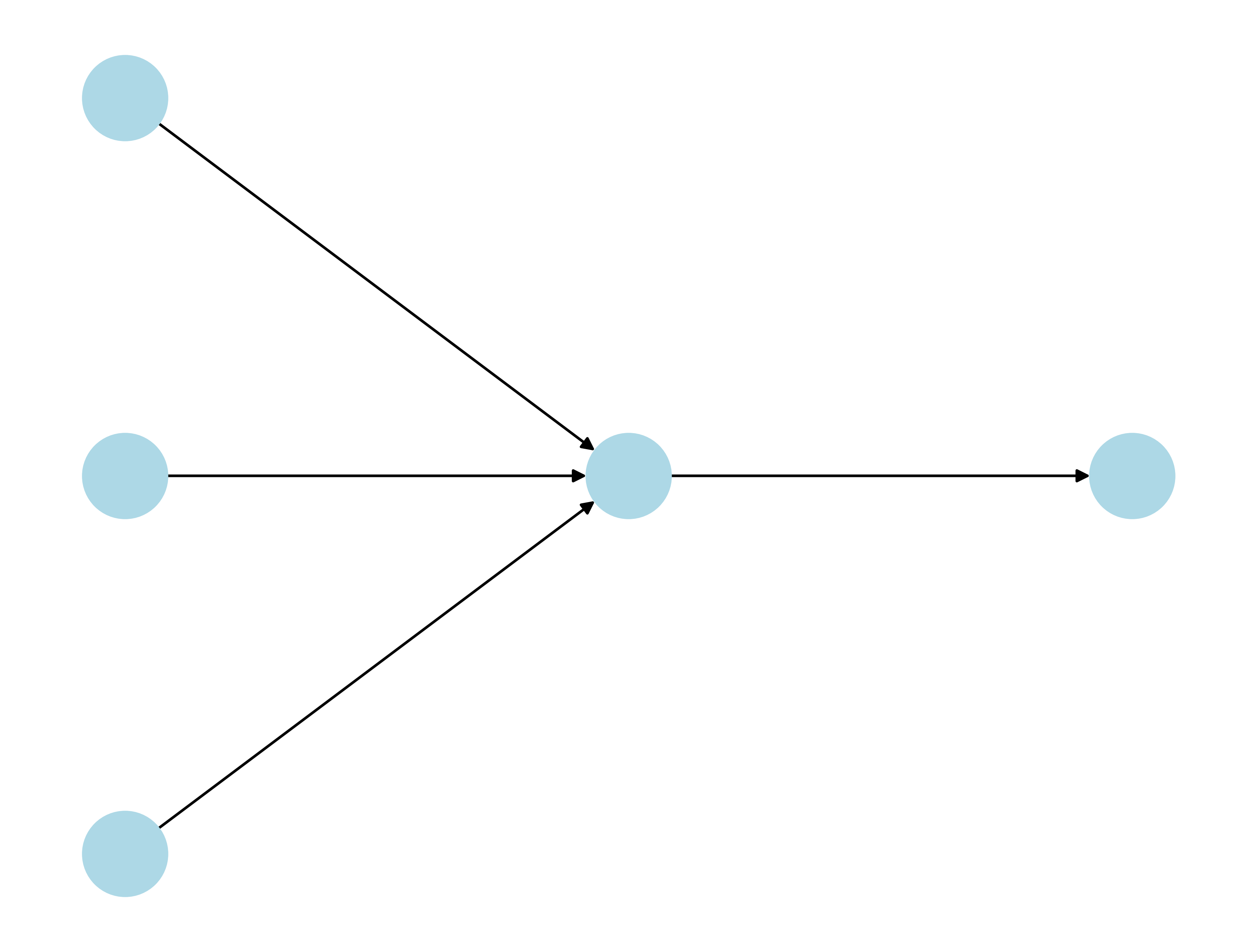
Referring to the nodes and arrows from left to right:
- First “Input” Layer of Nodes: 3 features (\(x_i\)’s)
- First Set of Arrows: 3 weights (\(w_i\)’s)
- Second “Hidden” Layer: computes \(\sum\limits_{i=1}^{3}w_ix_i + b\)
- Last “Output” Layer: returns the result \(z\)
The issue is that the output is an unbounded real number. For a binary classification problem where the output should be either 0 or 1, this doesn’t bode well. Activation functions account for this by bounding the output. There are plenty of choices for activation functions, each with their own strengths and use cases. Some of the most common activation functions include:
- Sigmoid
- Tanh (Hyperbolic Tangent)
- ReLU (Rectified Linear Unit)
The Sigmoid works well for binary classification problem with its ability to “squeeze” \(z\) between 0 and 1.
Sigmoid Function
\[g(z) = \frac{1}{1 + e^{-z}}\]
Using the Sigmoid activation function works like this:
- First “Input” Layer of Nodes: 3 features (\(x_i\)’s)
- First Set of Arrows: 3 weights (\(w_i\)’s)
- Second “Hidden” Layer: computes \(z=\sum\limits_{i=1}^{3}w_ix_i + b \rightarrow g(z)\)
- Last “Output” Layer: returns the result \(\hat{y} = g(z)\)
Feedforward, Loss Functions, Backpropagation, and Gradient Descent
How does a neural network actually work and how does it improve its predictions?
- Feed Forward: propagate information through network from input to output:
- Obtain Predition \(\hat{y}\)
- Loss Function: calculate loss compared to known labels (i.e., supervised machine learning), also known as error or cost. Quite a few options to obtain error between \(y\) and \(\hat{y}\). Some popular choices are:
- Mean Squared Error (MSE)
- Binary Cross Entropy (BCE)
- Categorical Cross Entropy (CCE)
- Backpropagation: from output to input (hence back), calculate the partial derivates for the cost function with respect to the parameters and layers:
- \(\nabla C = [\frac{\partial C}{\partial W_1}, \dots, \frac{\partial C}{\partial W_L}, \frac{\partial C}{\partial b_1}, \dots, \frac{\partial C}{\partial b_L}]\)
- Where \(W_i\) and \(b_i\) are weights and biases, respectively, for layer \(i \in [1, \dots, L]\)
- \(L\) is the output layer
- Gradient Descent: Update the weights and biases with a learning rate (\(\alpha\)) multiplied by the partial derivates.
- Iterate, Iterate, Iterate…: Repeat this process many times. Each iteration is known as an epoch. Ultimately, the goal is to have the cost continuously reducing on each epoch, eventually converging to a minimum (hopefully close to 0).
The steps above is a general overview of Neural Networks work, and is not exhaustive. A slightly more comprehensive network, but still pretty small can be imagined for a simple approach.
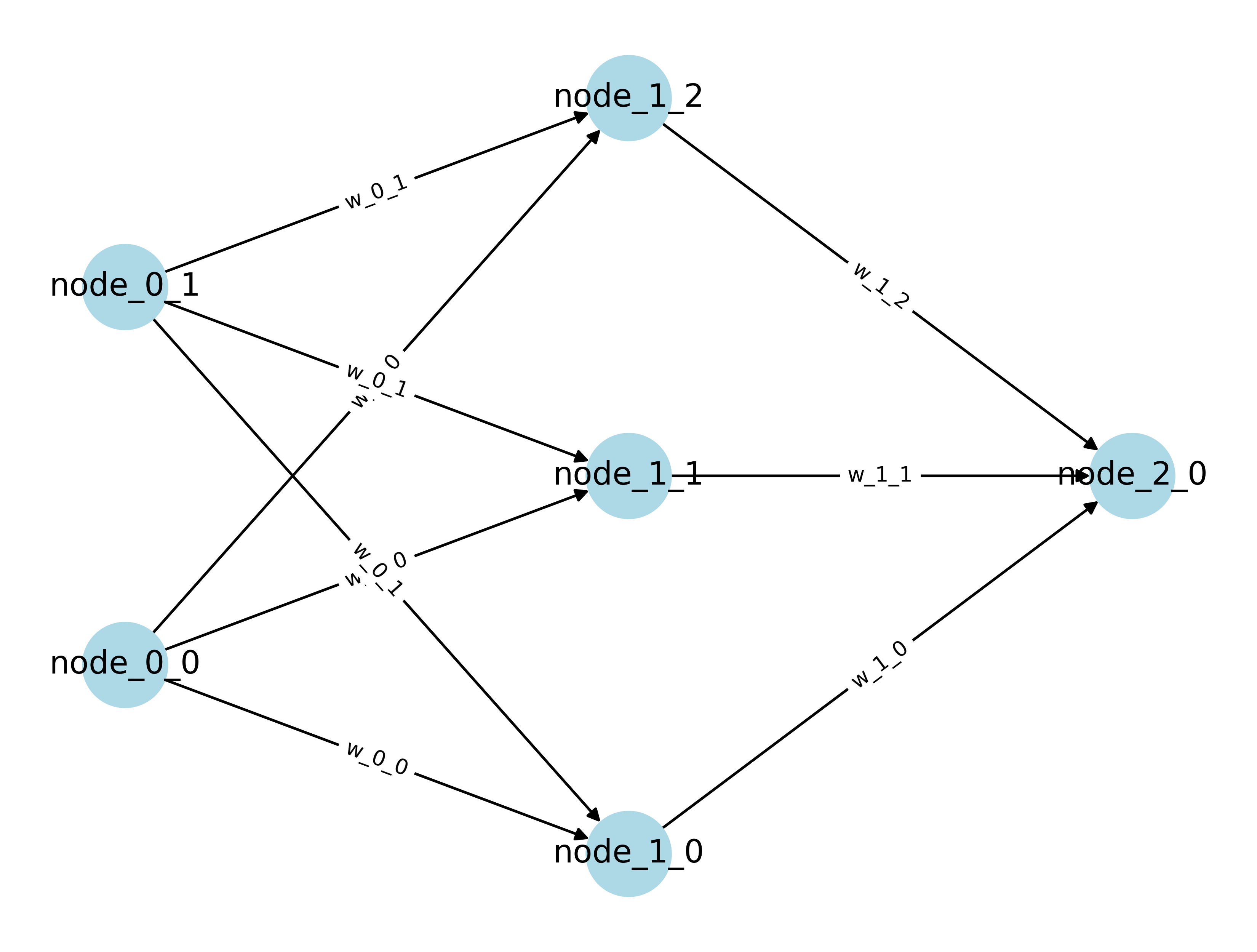
However, the idea is that neural networks can tackle much more complex problems that traditional statistical and machine learning models fall short on.
Acknowledgements
This project utilized a comprehensive guide for the mathematics and programming concepts of building a binary classification neural network model using a Sigmoid activation function with Binary Cross Entropy [3]. The concepts presented in the article were extended.
Data Preparation
This analysis focused on using a bespoke neural network to classify political bias within news articles. In particular, it used articles from media organizations with known Left or Right political bias. Neural Networks are a supervised machine learning method. Supervised Machine Learning models require labeled data, or known tags on the data to train the model. Additionally, when teaching the models, the data is split into disjoint training and testing sets. In essence, the models learn from the training set and then are tested on unseen data. This helps to prevent overfitting and simulates applying the model on real-world data.
Samples and sometimes full datasets (depending on size) can be found here.
Starting Data
A sample of the data used is seen below. The columns shown have the url of the news article, political bias of the news organization, the raw article, and the cleaned article after processing. This was the data scraped from NewsAPI and labels obtained from AllSides. Processing included:
- General HTML Token Removal
- Lowercasing
- Removing Links and Email Addresses
- Ensuring no Emojis or Accent Characters
- Expanding Contractions
- Removing Punctuation
- Removing Numbers and Words that Contain Numbers
- Removing Stopwords
- Lemmatizing
Vectorized Data
Using the cleaned column (as described above), the data was vectorized with CountVectorizer from sklearn using a limit of 1000 maximum features, and then reduced to the rows with the appropriate political biases of Left and Right. Additionally, the label was mapped to a binary representation with \(Left \rightarrow 1\) and \(Right \rightarrow 0\).
| BIAS | ability | able | academic | acceptance | access | according | account | act | acting | action | activity | actually | ad | add | added | adding | addition | additional | additionally | address | administration | administrative | advantage | affect | affected | affordable | age | agency | agenda | agent | ago | agreement | agricultural | agriculture | ahead | ai | aid | aim | air | allow | allowed | allowing | allows | amazon | vance | various | versus | vice | video | view | virginia | vote | voter | vought | want | wanted | war | washington | watch | water | way | wealth | website | wednesday | week | went | west | white | win | wing | wo | woman | won | word | work | worked | worker | workforce | working | world | worried | worth | wrote | year | yes | yield | york | young | yoy |
|---|---|---|---|---|---|---|---|---|---|---|---|---|---|---|---|---|---|---|---|---|---|---|---|---|---|---|---|---|---|---|---|---|---|---|---|---|---|---|---|---|---|---|---|---|---|---|---|---|---|---|---|---|---|---|---|---|---|---|---|---|---|---|---|---|---|---|---|---|---|---|---|---|---|---|---|---|---|---|---|---|---|---|---|---|---|---|---|---|---|
| Loading ITables v2.3.0 from the internet... (need help?) |
The vectorized dataset will be used in a PCA model for initial testing of the bespoke neural network and then in its entireity across the 1000 features.
Ten Feature PCA
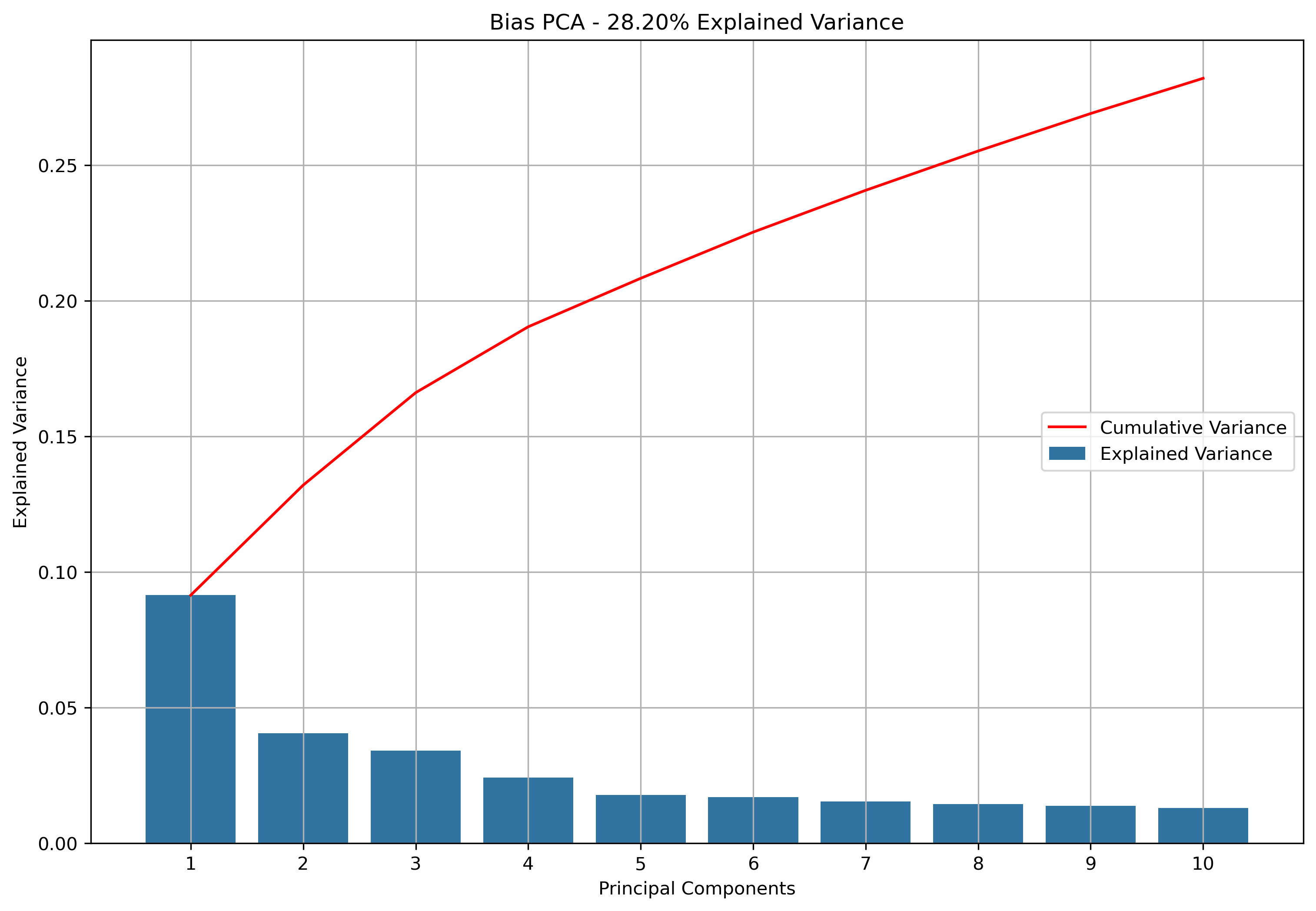
To get an idea if the custom built neural network could perform, a dataset with 10 features was used. This vectorized data was scaled and then reduced with 10-component PCA.
PCA Step
Ten principal components retained 28.2% of explained variance of the vectorized data.
Test Train Split Step
The data was then split into training and testing sets. As explained above, these are disjoint to simulate real world data.
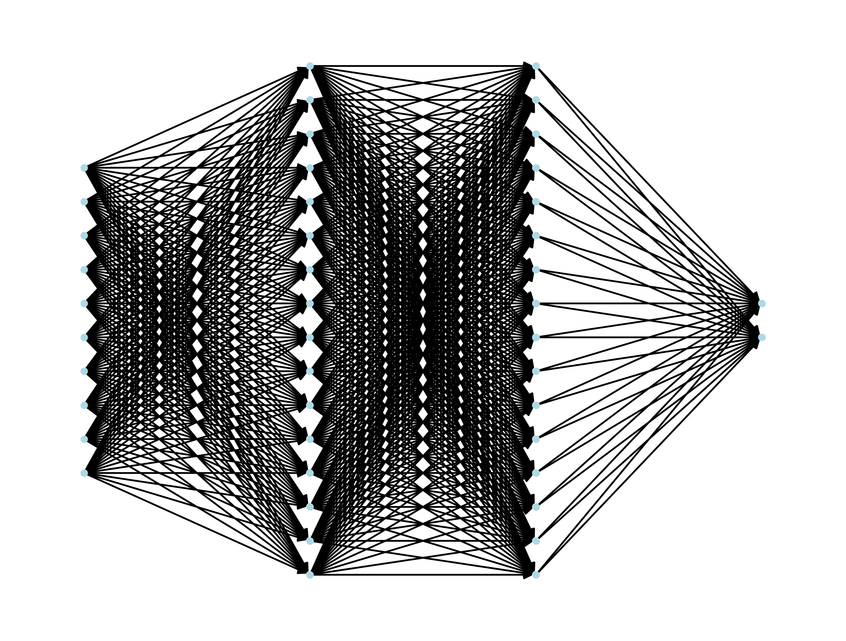
One Thousand Feature Count Vectorized
After proving the custom built neural network could perform, the neural network was further tested with the full 1000 feature vectorized dataset. The data was split into training and testing sets. As explained above, these are disjoint to simulate real world data.
Training Label
| BIAS | |
|---|---|
| Loading ITables v2.3.0 from the internet... (need help?) |
Training Data
| ability | able | academic | acceptance | access | according | account | act | acting | action | activity | actually | ad | add | added | adding | addition | additional | additionally | address | administration | administrative | advantage | affect | affected | affordable | age | agency | agenda | agent | ago | agreement | agricultural | agriculture | ahead | ai | aid | aim | air | allow | allowed | allowing | allows | amazon | america | vance | various | versus | vice | video | view | virginia | vote | voter | vought | want | wanted | war | washington | watch | water | way | wealth | website | wednesday | week | went | west | white | win | wing | wo | woman | won | word | work | worked | worker | workforce | working | world | worried | worth | wrote | year | yes | yield | york | young | yoy | |
|---|---|---|---|---|---|---|---|---|---|---|---|---|---|---|---|---|---|---|---|---|---|---|---|---|---|---|---|---|---|---|---|---|---|---|---|---|---|---|---|---|---|---|---|---|---|---|---|---|---|---|---|---|---|---|---|---|---|---|---|---|---|---|---|---|---|---|---|---|---|---|---|---|---|---|---|---|---|---|---|---|---|---|---|---|---|---|---|---|---|---|
| Loading ITables v2.3.0 from the internet... (need help?) |
Testing Label
| BIAS | |
|---|---|
| Loading ITables v2.3.0 from the internet... (need help?) |
Testing Data
| ability | able | academic | acceptance | access | according | account | act | acting | action | activity | actually | ad | add | added | adding | addition | additional | additionally | address | administration | administrative | advantage | affect | affected | affordable | age | agency | agenda | agent | ago | agreement | agricultural | agriculture | ahead | ai | aid | aim | air | allow | allowed | allowing | allows | amazon | america | american | angeles | announced | announcement | annual | answer | ap | app | application | apply | approach | approved | area | art | article | ask | asked | asset | assistance | associated | association | attack | attempt | attorney | authority | available | average | avoid | away | bad | balance | transgender | treasury | treatment | tried | trillion | trump | try | trying | tuesday | tuition | turn | type | typically | ultimately | uncertainty | unclear | undergraduate | understand | union | united | university | update | usaid | use | used | user | using | valuable | value | vance | various | versus | vice | video | view | virginia | vote | voter | vought | want | wanted | war | washington | watch | water | way | wealth | website | wednesday | week | went | west | white | win | wing | wo | woman | won | word | work | worked | worker | workforce | working | world | worried | worth | wrote | year | yes | yield | york | young | yoy | ||
|---|---|---|---|---|---|---|---|---|---|---|---|---|---|---|---|---|---|---|---|---|---|---|---|---|---|---|---|---|---|---|---|---|---|---|---|---|---|---|---|---|---|---|---|---|---|---|---|---|---|---|---|---|---|---|---|---|---|---|---|---|---|---|---|---|---|---|---|---|---|---|---|---|---|---|---|---|---|---|---|---|---|---|---|---|---|---|---|---|---|---|---|---|---|---|---|---|---|---|---|---|---|---|---|---|---|---|---|---|---|---|---|---|---|---|---|---|---|---|---|---|---|---|---|---|---|---|---|---|---|---|---|---|---|---|---|---|---|---|---|---|---|---|---|---|---|---|---|---|---|---|---|
| Loading ITables v2.3.0 from the internet... (need help?) |
Modeling
For both datasets, the neural network was ran across a grid with different architecture options. The differences were in the number of layers and number of nodes in the layers. They were all ran with \(10,000\) epochs and a learning rate of \(\alpha = 0.001\). After the grid search step, the best model was reran to obtain more metrics and examine convergence and overfitting.
The architectures were structured as [input, hidden layer 1, …, hidden layer L, output]:
- Architecture 1: [10, 16, 1],
- Architecture 2: [10, 32, 1],
- Architecture 3: [10, 64, 1],
- Architecture 4: [10, 128, 1],
- Architecture 5: [10, 16, 16, 1],
- Architecture 6: [10, 32, 32, 1],
- Architecture 7: [10, 64, 64, 1],
- Architecture 8: [10, 128, 128, 1],
- Architecture 9: [10, 16, 16, 16, 1],
- Architecture 10: [10, 32, 32, 32, 1],
- Architecture 11: [10, 64, 64, 64, 1],
- Architecture 12: [10, 128, 128, 128, 1]
PCA Results
Grid Search
| Architecture | Train Accuracy | Train Cost | Train Time | Test Accuracy | Test F1-Score |
|---|---|---|---|---|---|
| Loading ITables v2.3.0 from the internet... (need help?) |
Selected Architecture
Given the accuracy on the actual testing data, Architecture 5 performed the best in the grid search. Recall this only uses the Sigmoid activation function with Binary Cross Entropy, and doesn’t have features involving batches or dropout.
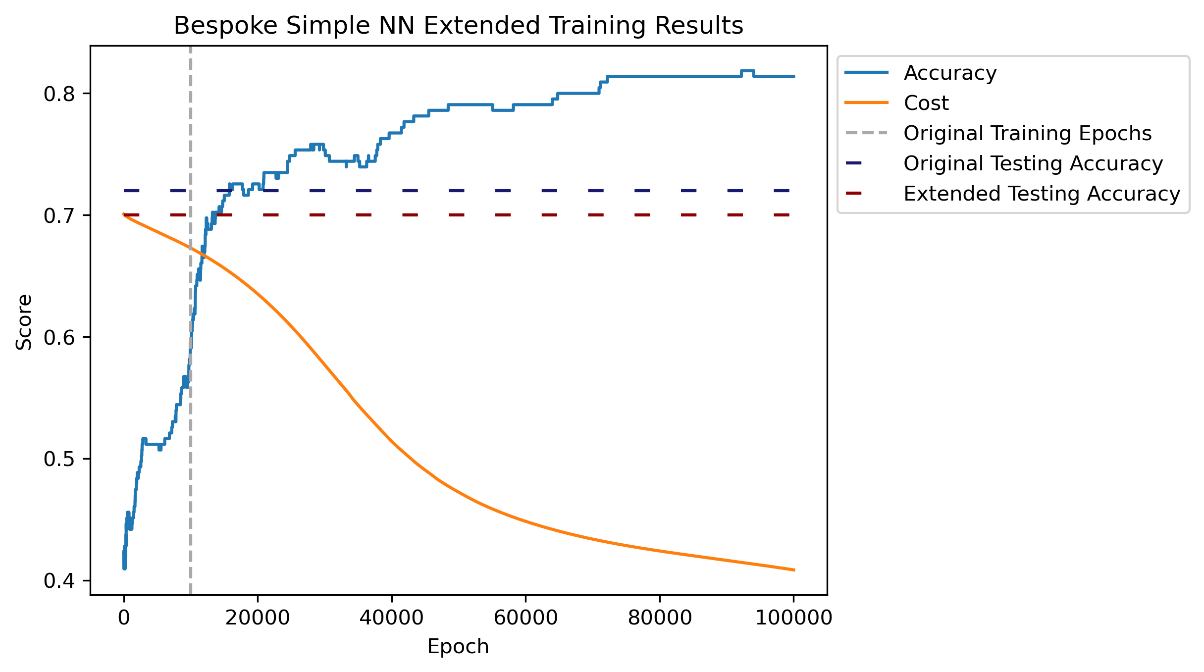
The selected model was ran for \(100,000\) epochs to investigate convergance and overfitting. Accuracy in the plot is calculated respective to the training data. Another \(90,000\) epochs does show a slightly converging accuracy, but cost looks like it hasn’t leveled out. There is an aspect of overfitting occuring, as the extended training accuracy has a slight reduction compared to the original set.
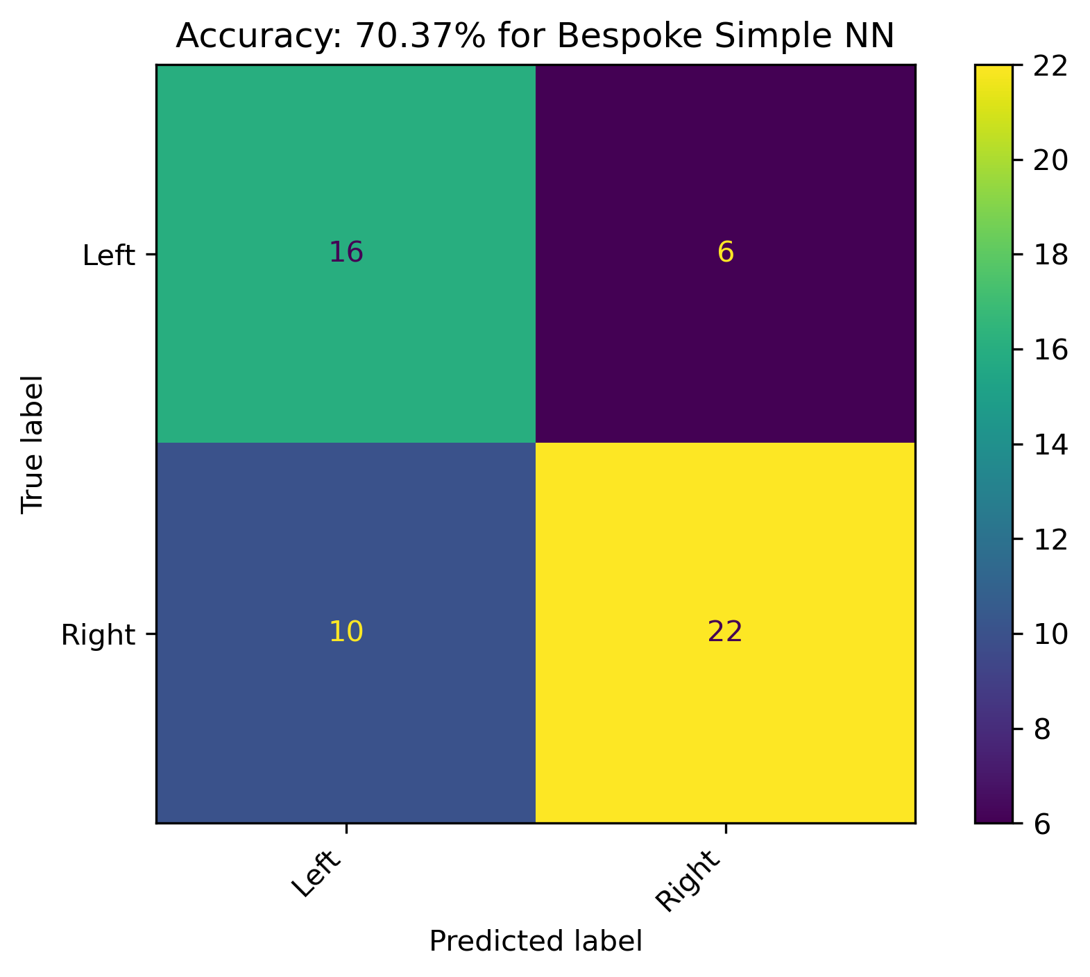
This final model resulted in an accuracy of just over 70%, with the majority of incorrect predictions stemming from predicting Left when the label was actually Right.
Full Results
Grid Search
| Architecture | Train Accuracy | Train Cost | Train Time | Test Accuracy | Test F1-Score |
|---|---|---|---|---|---|
| Loading ITables v2.3.0 from the internet... (need help?) |
Selected Architecture
Given the accuracy on the actual testing data, Architecture 1 performed the best in the grid search. Recall this only uses the Sigmoid activation function with Binary Cross Entropy, and doesn’t have features involving batches or dropout.
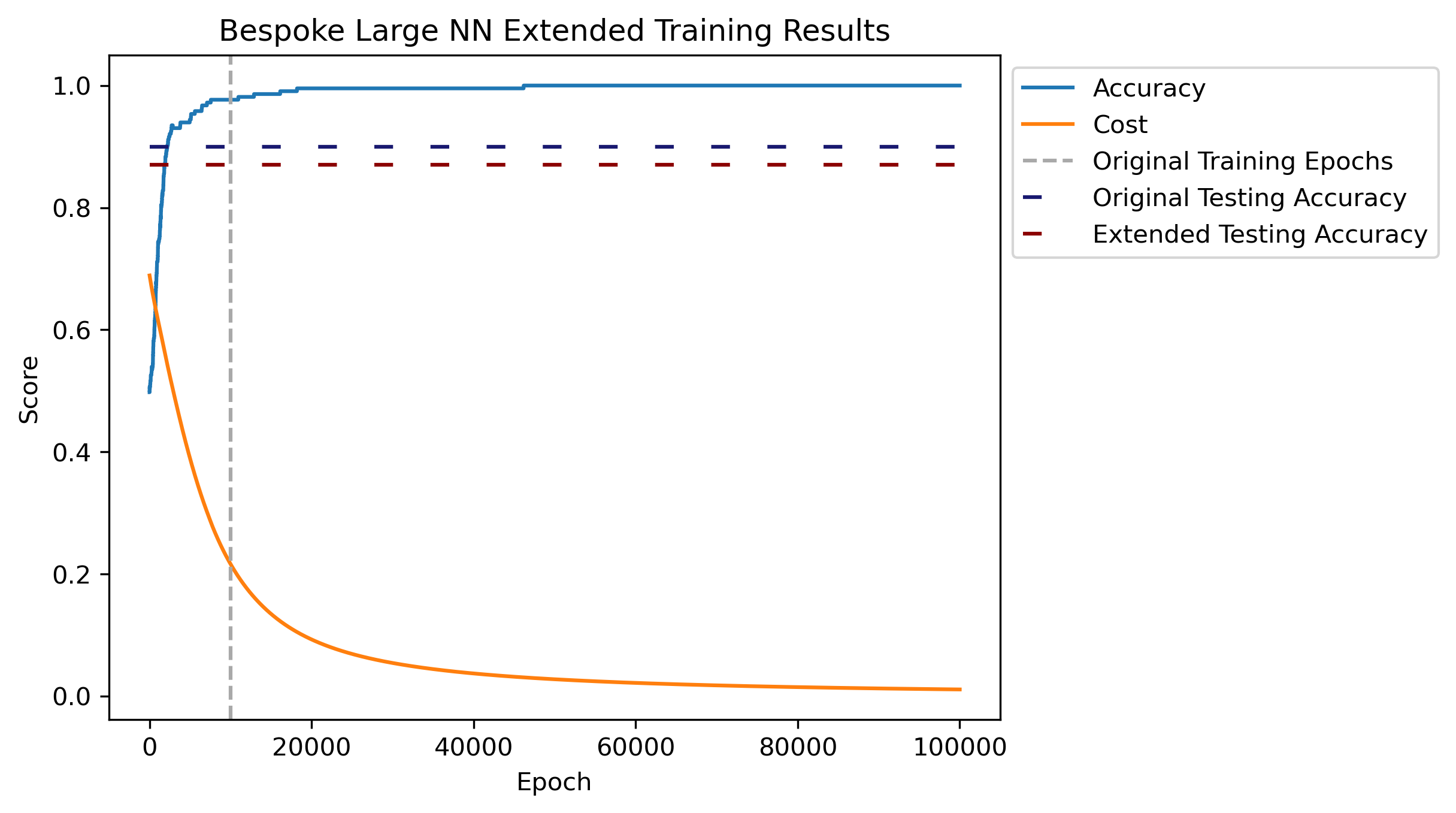
The selected model was ran for \(100,000\) epochs to investigate convergance and overfitting. Accuracy in the plot is calculated respective to the training data. Another \(90,000\) epochs does show a more distinct convergence for both accuracy and cost. There is an aspect of overfitting occuring, as the extended training accuracy has a slight reduction compared to the original set. Although it still respectable.
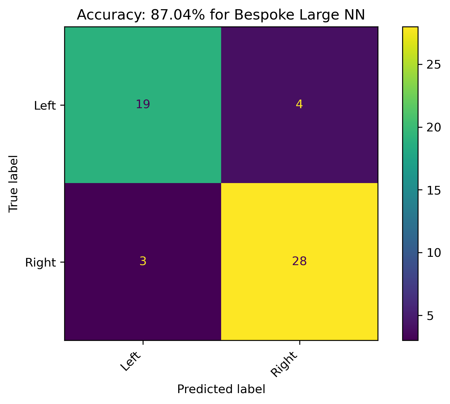
This final model resulted in an accuracy of just over 87%, with an almost balanced handful of incorrect predictions for both labels.
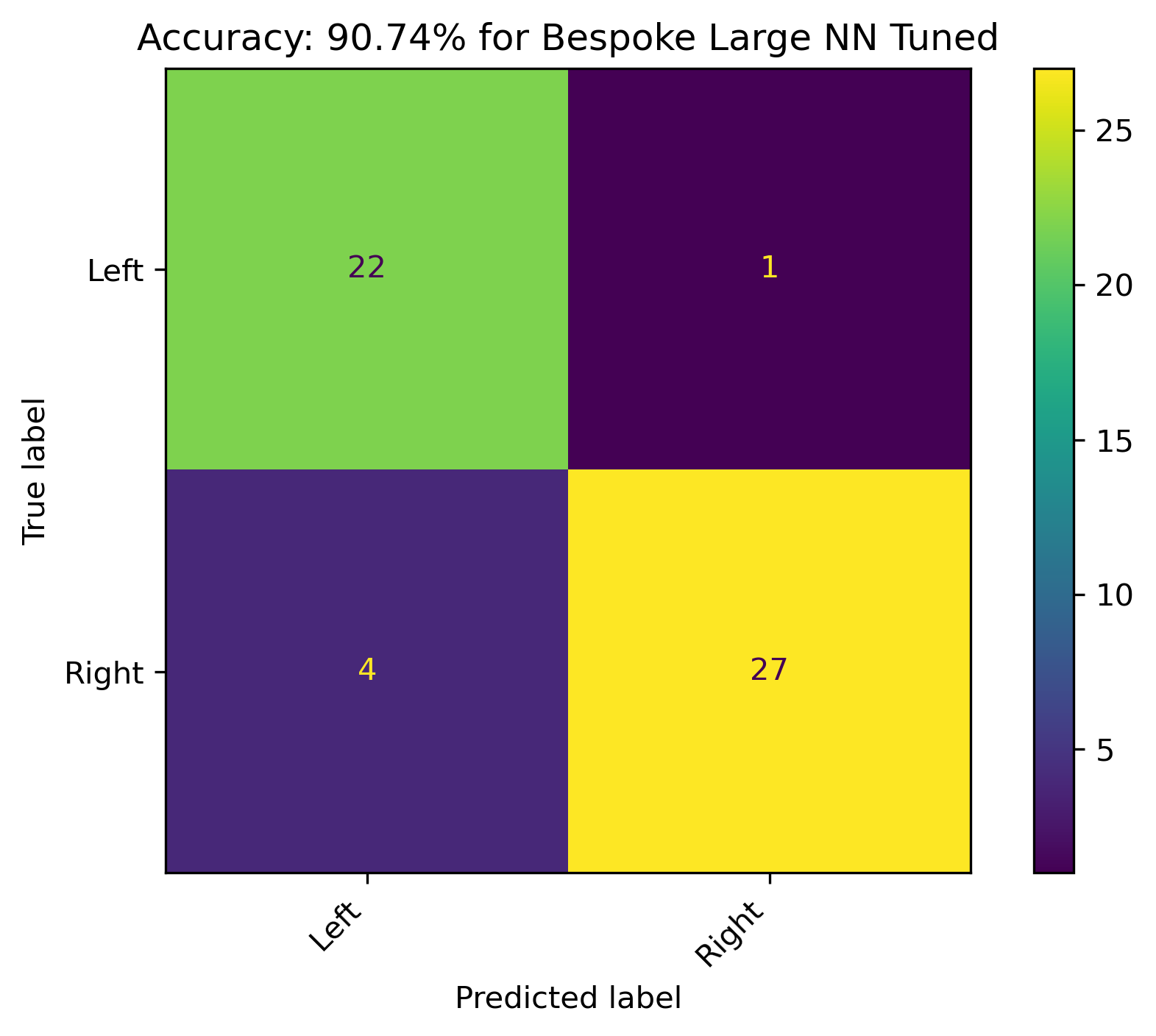
The Final Run
Since the accuracy and cost converged adequately for the 1000 feature neural network, another model was ran for the number of epochs where the accuracy with respect to the training data start to level out, \(20,000\) epochs. This seemed to address the overfitting, resulting in an accuracy of over 90% for the actual testing data.
Conclusion
News articles published by organizations with known political biases were modeled in an attempt to project political bias on text content when it is unknown. Although political bias can vary between authors and news topics within a single organization, a model which does well with a high amount of complexity was used in this attempt.
A network based model was used used in an attempt to predict the biases of Left or Right categories of an article. Two varieties of the news articles were used. The first variety reduced the news articles from 1000 high frequency words to a few features with a method known for retaining as much information as possible within these features. The second variety used these 1000 high frequency words by counting their appearances in the articles.
In this case, using the reduced features resulted in a moderate prediction accuracy of just above 70%, while the prediction accuracy was just above 90% when using the larger amount of features. Although the process for producing the 90% accuracy model had a higher computational cost, it created robust and effective results.
It should be noted that this was a rather simple version of a network based model. This family of models can be highly efficient at uncovering complex patterns across massive amounts of data. Given more data and further production on the bespoke network model, there is potential for further improvements.
Code Links
References
1.
Datamapu (2023) A Brief History of Neural Nets — pub.towardsai.net
2.
GeeksforGeeks (2024) How Neural Networks Solve the XOR Problem - GeeksforGeeks — geeksforgeeks.org
3.
Mallick A (2024) Learn to Build a Neural Network From Scratch — Yes, Really. — waadlingaadil